A Unified Theory of Brain Sensing
There are many ways to measure brain activity from outside the head1: EEG, MEG, fMRI, fNIRS, ultrasound, and more. How would you go about comparing them, quantitatively?
People usually start with resolution, analogous to the pixel density in a camera sensor. But if you know about cameras, you know that the number of megapixels in your camera is far from a complete picture of how good your camera is.
The especially weird thing about resolution for brain imaging is that a global resolution is not even well defined, which is why so many papers disagree on the resolution of the same modality. The resolution depends on the depth you're considering, the assumptions you make about the signal, like whether it's sparse or not, and what algorithms you use to reconstruct your brain images.
What we really care about is information: how many bits per second can this device tell you about what's going on in the brain? In this post, we'll compute, from first principles, the theoretical information limit of all the popular brain imaging modalities.
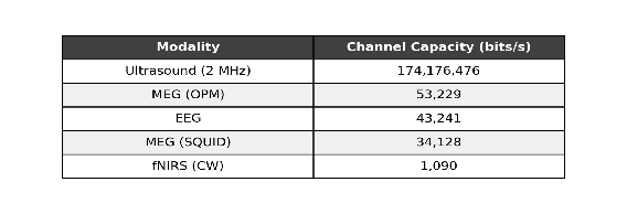
The spoiler is we get a table like this:
| Modality | Today bit/s | Today noise floor | Today config | Limit bit/s | Limit noise floor | Limit config |
|---|---|---|---|---|---|---|
| MEG OPM | — | — | — | — | — | — |
| MEG SQUID | — | — | — | — | — | — |
| EEG | — | — | — | — | — | — |
| fNIRS CW | — | — | — | — | — | — |
| fMRI BOLD | — | — | — | — | — | — |
| Ultrasound | — | — | — | — | — | — |
And plots that show how the information scales with the number of sensors:
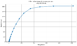
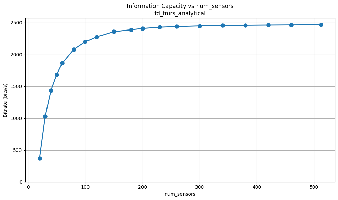
We'll explain how we get this and show scaling plots showing how the information scales with the number of sensors.
But first some observations:
"Just add more sensors and it'll work"
There's a narrative that the reason EEG doesn't work well is that it doesn't have enough sensors. Our plots show that adding more sensors to EEG past about 500 sensors does not help.
EEG and MEG have roughly the same information content
Brain sensing as a communication channel
Each imaging modality can be viewed as a communication channel between the brain and the sensors. The device transforms the state of the brain — for example, which neurons are firing and when — into measurements such as voltages on EEG electrodes, magnetic fields in MEG, etc. in a way constrained by physics.
The human brain has about 100 billion neurons. So let's represent the state of the brain as a 100-billion-dimensional vector x, where each element encodes whether a neuron is firing in a given millisecond.
Then we can write the transformation from brain state to measurements, y, as some function
In practice, our sensors aren't perfect, so we also add noise.
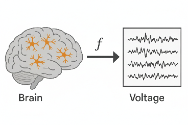
You can think of the vector y as, for example, voltage measurements for each electrode in EEG. f is a physical simulator of the modality; it tells you, in the absence of noise, what measurements you'd get for a given brain state. We call f the forward model.
How do we get the forward model f? We'll explain that later, but the rough idea is that there are equations from physics that you can use to model each modality. Then you can write a simulator that solves those equations.
Let's go back to our original goal of measuring information. What we're trying to do is study the function f, and ask how much of the brain state is actually represented in the measurement, and how much gets lost.
For most imaging modalities, the variations in x are small enough that the function is close to linear2, so we can represent the function f as a matrix, A.
So now it becomes a linear algebra problem! The linear algebra question we're asking is something like "how invertible is the matrix?" If it's invertible, then you can perfectly recover the brain state from the measurements.
Matrix inversion in the real world
Usually in linear algebra, you think of matrix inversion as a binary thing — either the matrix is invertible or it's not. But it's actually more of a continuous thing once you move to the real world, where you have noise in your measurements.
The less binary way of asking how invertible a matrix is, is by looking at its singular values.
The singular value decomposition (SVD) gives you a way to decompose the brain state x into components (called singular vectors), and the singular value tells you how much each component gets amplified or attenuated in your measurement. Think of each singular value as a gain in an amplifier circuit. For example, if the i'th singular value is 0, that means all the information in x related to the i'th singular vector gets lost. But it's not binary. If the singular value is very small, that part of the measurement will also get drowned out in noise.
Let's take an example of blurring a signal. Here's the singular value spectrum of a Gaussian blur. In these spectrum plots, we sort the singular values from largest to smallest.
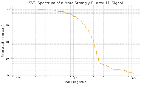
You see that initially the spectrum is high, but then it drops off exponentially. So when you blur a signal x, there are components of that signal that get very strongly attenuated. Let's look at what those components look like.
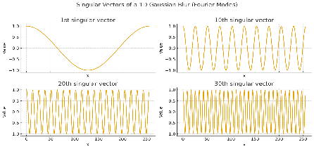
The early singular vectors are low frequency, whereas the high ones oscillate a lot. So blurs attenuate pieces that oscillate a lot. This makes sense: if you blur an image with sharp edges (i.e. the neighboring pixels change drastically), the sharp edges go away.
The idea that the early singular values are the low resolution parts and the late ones are the high resolution parts will generalize to brain imaging.
Fun math fact An interesting fact is that the singular vectors of a blur are precisely the Fourier basis vectors and the singular values are equal to the Fourier transform of the signal.
Can you undo a blur?
If you have no noise, the answer is actually yes! With perfect knowledge of the forward model (in our case, the precise degree of blurring represented by the width of the Gaussian), since the singular values don't go to 0, we can invert the matrix, and get back the unblurred signal. So in the noiseless case, you haven't lost any information!
The problem is when you add noise. The picture is like this:
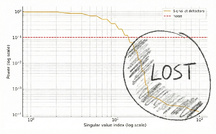
In the early components, the signal lies above the noise. But after some singular value, the components get drowned out by noise. So after blurring, you have forever lost the small singular value pieces of your signal.
Why is the noise a flat line? We assume the noise is independent and identically distributed across detectors (see the Noise section below for why this is true). In this case, the variance of the values ⟨n, u_i⟩ will be the same for all singular vectors u_i.
But can't machine learning undo a blur? Isn't super-resolution a thing in machine learning? Yes! There's a field of machine learning known as super-resolution or upsampling. It seems like you can magically increase the resolution of images.
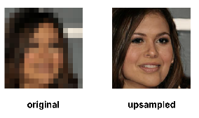
But the key to super resolution in machine learning is that you assume a prior over the possible signal vectors x. For example, you know that natural images are more likely than random noise, so you can guess the later singular components from the earlier ones. The later singular components are not giving you any more information, they are redundant.
But if your signal was truly random Gaussian noise, no machine learning method will recover it! The early components of x will not tell you anything about the late components of x.
Could machine learning super resolution be applied to brain imaging? Totally. And this is another reason we don't like the resolution metric. But the key is that machine learning cannot increase the channel capacity of the system.
SVDs of brain imaging modalities
We turned a bunch of brain imaging modalities into matrices, and computed the singular value decomposition of all of them.
Here's the singular value spectrum of all of them, normalized by their first singular value.
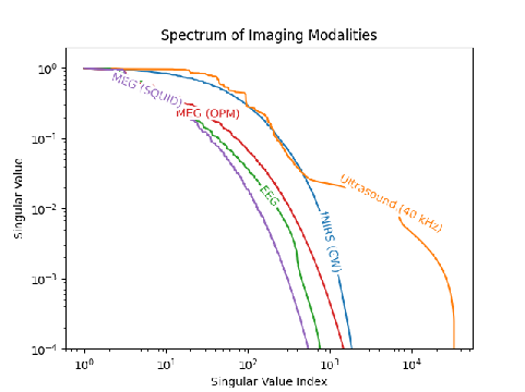
We can see that modalities like EEG and MEG fall off much more quickly than fNIRS and ultrasound. Critically though, this is for a single time sample, and doesn't include the temporal dynamics where EEG and MEG shine (more on that later).
For MEG, the singular vectors can be visualized directly: the right singular vector is the pattern of brain sources, and the left singular vector is the detector pattern that source mode produces. Because the leading MEG gains are close together, the exact numbering of modes 1-3 can rotate with a different grid; the paired source/detector subspace is the stable object.
How many sensors do you use for each modality? These spectra actually represent the case where you have infinite sensors! Of course, you can't simulate infinite sensors on a computer, but we ran scaling experiments which showed convergence in the spectrum.
How do you simulate a brain imaging modality? What does that even mean? Each modality is governed by partial differential equations which describe its physics.
For example, in fNIRS, you send near-infrared light through the brain. If you know how much each point in the head scatters and absorbs light, you can predict where the light will go. The equation which describes this is called the Radiative Transfer Equation, and is actually also used to model nuclear reactors!
Once you have equations for the physics, you can compute the derivative of the sensor readings with respect to the brain properties (either analytically or with a differentiable partial differential equation solver). These derivatives give you the matrix A for each modality.
All our experiments were done on a simple model of the head. We model the head as a hemisphere with 3 layers — scalp, skull, and brain.
Here's a table of the equations used for each modality:
| Modality | Differential equation | Package used | Head properties assumed |
|---|---|---|---|
| EEG | Poisson equation | OpenMEEG | Conductivity of brain = conductivity of scalp = 33× conductivity of skull |
| MEG | Biot-Savart | Analytical (Sarvas formula) | — |
| fMRI | Reconstructed BOLD image model | Analytical Gaussian PSF + HRF | 1% BOLD contrast, finite voxel size, temporal HRF |
| fNIRS | Radiative transfer equation | Analytical Green's function | Homogeneous absorption and scattering coefficients |
| Ultrasound | Acoustic wave equation | Analytical Green's function | — |
There was a ton of detail and engineering needed to compute these SVDs. A single simulation could take hours to run, even on a GPU, and the matrices A had up to 100 billion elements — on the same scale as the number of parameters in a large language model! To run SVD on such large matrices, we had to write our own SVD implementation that ran on multiple GPUs.
The noise
To compare the modalities, we also need to estimate the noise in each modality. It's unfortunately physically impossible to have zero noise for each of the modalities we're considering.
Let's take EEG as an example. EEG measures the voltage on the head. But because the brain is not at absolute zero, charges in the brain will move randomly, and those random movements will lead to non-neural voltage readings in your sensor! Crucially, this will appear even if you spend a gazillion dollars to have a "perfect" EEG sensor. For EEG, this noise is called Johnson noise.
There are similar fundamental noise sources in other modalities as well. In fNIRS, you can only send so many photons into the brain before your head absorbs so much energy that it starts to cook, and the detectors will therefore suffer from shot noise limits due to measuring finite photons.
Here's a table of the noise sources for each modality:
| Modality | Fundamental noise | Today's best | Noise limit |
|---|---|---|---|
| EEG | Johnson noise | ~90 nV (5 kΩ, 100 Hz BW) | Same — thermodynamic floor |
| MEG SQUID | SQUID flux noise | 5 fT/√Hz | 0.1 fT/√Hz (body thermal) |
| MEG OPM | Atomic spin noise | 15 fT/√Hz | 0.5 fT/√Hz (spin projection, 1 cm³ cell) |
| fMRI | Thermal/reconstruction + physiological noise | BOLD response SNR derived from 1% contrast and tSNR ~80 | high-quality BOLD response SNR floor |
| fNIRS | Shot noise | 62 ppm (5 mW) | 23 ppm (ANSI max, 35 mW) |
| Ultrasound | Acoustic thermal modal power | frequency-dependent | Same — thermodynamic floor |
Each of these noise sources are additive, Gaussian, and independent across the sensors.
Channel capacity
The SVD lets us model the signal and we now have an understanding of the noise. Let's fuse them together to compute the maximum information transmissible for each modality.
Every communication channel has a limit to how much information can be sent through it. It's called the channel capacity. If the noise is Gaussian and uncorrelated in time, you can write a precise mathematical expression for the channel capacity. For each sample, it's
Since we have many sensors and many neurons, we have many communication channels. Unfortunately, you can't just sum the information content between each neuron–sensor pair because the information is not independent.
The SVD gives us a way to decompose the communication into independent channels. Since each singular vector is orthogonal to the others, and the noise is assumed to be independent between sensors, we can compute the information for each SVD component separately, then sum them together.
where n is the noise at the sensors, and a_i is the magnitude of the source's i'th singular component. Since we don't make assumptions on which SVD channels the brain will communicate on, we use an algorithm called the water-filling algorithm which smartly picks how much of the signal power to put in each component to maximize the information transfer.
For the first-principles estimates below, we use the physical detector-floor path: detector noise divided by source amplitude. The interactive explorer also exposes an empirical observed-SNR mode, which is useful as a sanity check but normalizes away the absolute forward-model gain.
And that's it! That's how we compute the channel capacities for each modality.
The beauty of this method is that it only requires knowledge of the physics of the modality. It can evaluate systems that don't exist yet — including systems that would cost many millions of dollars to build — and make predictions for how a system with more sensors or lower noise would behave.
Interactive scaling explorer
How does information capacity scale with the number of sensors and source resolution for each modality?
Limitations
Despite the ambition of the title, the maximal information rate won't be the end-all-be-all metric for brain imaging. If you need an imaging modality with very low latency, contrast-free ultrasound shouldn't be your top choice. But for tasks that are sufficiently general, and need to measure from large parts of the brain, we think this framework provides a principled comparison.
Temporal dynamics. In the Gaussian blur example, as well as in most of the computations, we've assumed a stationary system and one sample from it. What you actually get in reality is a recording on each sensor over time. If you assume each time point is independent from each other, the SVD spectrum of the resulting measurement operator consists of the same values, repeated for each time point.
Footnotes
-
We focus in this post on brain imaging modalities, but the mathematical methods are very general and apply to any imaging problem, like observing the universe. ↩
-
For EEG & MEG, the forward model is linear. For ultrasound, the reflected signal is orders of magnitude weaker than the transmitted pressure, so secondary reflections are very small, and the problem is effectively linear. For fNIRS, the changes in μ_a are very small, such that the linear approximation fits the data well. Despite all this, even if the problem is not linear, the SVD spectrum of the linearized version should still tell you a ton about how much information is preserved. ↩